Surely every active PC user, at least once in his life, has come across the fact that when working in Microsoft Office Excel, it became necessary to hide some of the entered data without deleting it from the table. This can be done by simply hiding individual columns or rows. This feature of the program will be very useful when you need to preview a document to be sent to print.

I think many of you know how difficult it is to work with tables in which numbers creep into an endless canvas. In order to focus exclusively on the main values, to remove intermediate results from your eyes, the function of hiding unnecessary cells will come in handy. By the way, if in the process of checking the document you find flaws in it, you will have the opportunity to display the data hidden in the Excel sheet in order to correct it.
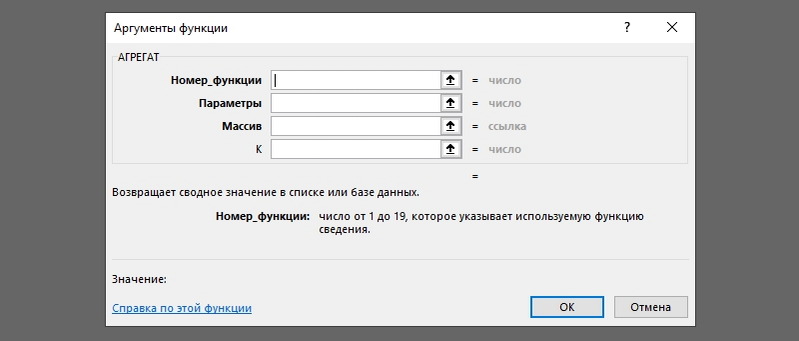
I should note that no formula that used data from hidden cells in the calculation will be cleared after you hide the cell with the original data. The fact that a value disappears from sight does not mean that it disappears from the table, and therefore your formulas, rest assured, will function normally. The only exception to this rule is an Excel function called Subtotals. The point is that if the value of the first argument of the specified function is greater than 100, then it will ignore all data that, as a result of structuring or filtering, ended up in hidden rows or columns. By the way, after the introduction of the new “Aggregate” function, Excel users have the opportunity to set a special parameter with which they can ignore the data of the cells that were hidden.
How do I hide data in columns and rows?
If you are faced with the need to hide columns and / or rows, then the following methods will certainly come in handy:
- Highlight the cells in the columns and / or rows that you need to hide. After activating the required area, go to the “Home” tab and select the “Cells” category in the drop-down list. Go to “Format”. A window should open in front of you, in which you will find the item “Hide or Show”. With a mouse click, select and activate the function you need – “Hide columns” or “Hide rows”, respectively.

- Select the columns and / or rows you do not need and by clicking on the right mouse button in the header area of the selected columns, call the context menu. In the window that appears, find and select the “Hide” command.

- Select the area with interfering cells that you want to hide, and then use the keyboard shortcut “Ctrl + 0” to remove columns, or “Ctrl + 9” if you want to get rid of the work area of rows.
How to show hidden data?
It is possible that soon after you hide the data you do not need, you will need it again. The developers of Excel provided for such a scenario, and therefore made it possible to display cells previously hidden from the eyes. In order to return the hidden data back to the visibility zone, you can use the following algorithms:
- Select all the columns and rows you have hidden by activating the Select All function. To do this, you will need the key combination “Ctrl + A” or click on the empty rectangle located to the left of the column “A”, immediately above the line “1”. After that, you can safely proceed to the already familiar sequence of actions. Click on the “Home” tab and select “Cells” from the list that appears. Here we are not interested in anything except the “Format” item, so you need to click on it. If you did everything correctly, you should see a dialog box on your screen in which you need to find the “Hide or Show” item. Activate the function you need – “Show columns” or “Show rows”, respectively.

- Make active all zones that are adjacent to the area of hidden data. Right-click on the blank area you want to display. A context menu will appear on your screen, in which you need to activate the “Show” command. Activate it. If the sheet contains too much hidden data, then again it makes sense to use the key combination “Ctrl + A”, which will select the entire workspace in Excel.

By the way, if you want to make column “A” available for viewing, then we advise you to activate it by typing “A1” in the “Name field” located immediately after the line with formulas.
It so happens that even performing all of the above actions does not have the desired effect and does not return hidden information to the field of view. The reason for this may be the following: the width of the columns is equal to the “0” mark or a value close to this value. To solve this problem, simply increase the width of the columns. This can be done due to the banal transfer of the right edge of the column to the distance you need to the right side.
In general, it should be recognized that such an Excel tool is very useful, since it provides us with the opportunity at any time to correct our document and send to print a document containing only those indicators that are really needed for viewing, without removing them from the workspace. Control over the display of the contents of cells is the ability to filter the main and intermediate data, the ability to concentrate on the priority problems.