Replacing numbers with words in Excel

Every user who has to work a lot with documents would like to simplify and automate their work at least to some extent. Special tools implemented by the developers in the Microsoft Excel spreadsheet editor allow you to do this. In this article, we will figure out how to convert a number to text in Excel and vice versa. Let’s get started. Go!

Converting a number to text

There are several ways to effectively solve the problem. Let’s take a closer look at each of them.

Formatting via the context menu

This is the most commonly used conversion option, so we decided to start with it. Follow the instructions below and you should be good to go.

1. First of all, select the values ​​on the sheet that you want to convert to text. At the current stage, the program interprets this data as a number. This is evidenced by the set parameter “General”, which is located on the tab “Home”.
2. Right-click on the selected object and select “Format Cells” in the menu that appears.
3. A formatting window will appear in front of you. Open the subsection “Number” and in the list “Number formats” click on the item “Text”. Then save the changes with the “OK” key.
4. After completing this procedure, you can verify that the conversion was successful by looking at the Number submenu in the toolbar. If you did everything correctly, a special field will display information that the cells have a text form.
5. However, the setup does not end in the previous step. Excel has not fully completed the conversion yet. For example, if you decide to calculate the autosum, then the result will be displayed just below.
6. In order to complete the formatting process, one by one, for each element of the selected range, do the following manipulations: make two clicks with the left mouse button on the cell and press the “Enter” key. Double pressing can also be replaced with the function button “F2”.
7. Ready! Now the application will perceive the numerical sequence as a text expression, which means that the autosum of this data area will be equal to zero. Another sign that your actions have led to the desired result is the presence of a green triangle inside each cell. The only thing is that in some cases this mark may be absent.

Tools in the ribbon

You can also change the data type in Excel using special tools located on the top panel of the program. This method consists in using the numeric block and the format display box, which we have already mentioned. The algorithm of actions is somewhat simpler than in the previous case. However, in order to avoid questions and difficulties, we have prepared a corresponding guide.

1. Select the desired range, and then go to the “Home” tab. Here you need to find the “Number” category and click on the small triangle next to the format field (the default is “General”).
2. In the drop-down list of options, select “Text” display type.
3. Then, as in the previous method, sequentially for the entire range, place the cursor on each cell and double-click LMB (or F2), and then click on the “Enter” key.

Using the function

An additional way to reformat numeric elements into text is the basic function “TEXT”. It is especially convenient to use in cases when you need to transfer values ​​with a new format to another column or the amount of data is too large to manually perform transformations for each cell. Agree, if a document has hundreds or even thousands of lines, conversion using the options already considered is not rational, since it will take too much time.

How to work with this option:

1. Select the cell where the converted range will start. Next, near the line with the formulas, click on the “Insert function” icon.
2. You will see the “Function Wizard” window. Here you need to select the category “Text” and in the field located just below, the corresponding item “TEXT”. Confirm with “OK”.
3. Next, a panel will appear with setting the arguments for the selected function, which consists of two parameters: “Value” and “Format”. In the first field, enter the number to convert, or provide a link to the place where it is located. The second field is for correcting non-integers. For example, if you write “0”, then the result will be without fractional signs, even though they were present in the source. Accordingly, if you write “0,0”, then the text type will have one digit after the decimal point. Similarly, what you see at the exit is formed if you enter “0.00” and the like.

Upon completion of all manipulations, click on the “OK” button.

4. Now you just need to copy the formula to adjacent sheet elements. To do this, move the cursor to the lower left corner of the cell you just edited. When the cursor changes to a small cross, hold down the left mouse button and drag the formula to the entire field of the range parallel to the original data.
5. As you can see, all the numbers have appeared in their places. However, the conversion process is not over yet. Select the resulting column and on the “Home” tab in the very first section “Clipboard” click on the “Copy” icon.
6. If you want to keep the initial version: without dropping the selection, right-click on the transformed area and select “Paste Special” in the offered list, and in the next window click on “Values ​​and Number Formats”.

In the event that you want to replace the original data with new ones, edit the original column. Paste in the same way as described above.

7. If you chose the second option, then the fragment with formulas can be deleted. To do this, select them, right-click → “Clear Content”.

Converting text to number

It’s time to consider ways to convert back to Excel. There are several more methods for converting textual data into numbers, so we are sure that you will find the most suitable one for yourself.

Conversion with error notification

One of the fastest and easiest ways to convert is to use a special icon that notifies the user of a possible error. This icon is shaped like a diamond with an exclamation point in it. It usually appears when you select cells that have a green checkmark in the upper left corner, which we talked about earlier. The numbers contained in the field with the textual representation arouse suspicions in the program, and thus it signals the user to pay attention to this moment. However, Excel does not always display this icon, so the formatting method under consideration is more situational. But in any case, if you find this “beacon” in yourself, you can easily perform the necessary transformations.

1. Click on the cell in which the error indicator is located, and then click on the corresponding icon.
2. In the menu that opens, select the “Convert to number” item.
3. After that, the object will immediately assume a numeric type.
4. If you need to reformat several values ​​at the same time, select the entire range and repeat the previous steps.

Format window

Excel also has the ability to convert back through a special formatting window. The algorithm is as follows:

1. Select the range of numbers presented in the text version, and then right-click.
2. In the context menu, we are interested in the “Format cells” item.
3. A formatting window will open, in which you need to make a choice in favor of one of two formats: “General” or “Numeric”. Regardless of which option you choose, the application will treat numbers as numbers. The only thing is that if you have selected the “Numeric” method, then in the right block you can additionally configure such parameters as the number of decimal places and place separators. After all the manipulations, click on “OK”.
4. At the last stage, you need to click through all the elements one by one by placing the cursor in each of them and pressing “Enter”.

Tools in the ribbon

Another fairly simple way to translate a textual data type into a numeric one is carried out using the tools located on the upper working panel.

1. First of all, you should highlight those values ​​that are to be transformed. Next, on the Quick Access Toolbar, go to the “Home” tab, and then on the ribbon, find the “Number” group.
2. In the special field set “General” view or “Numeric”.
3. After that, separately click on each of the selected cells using the “F2” and “Enter” keys. We have already described the algorithm above.

Formatting is complete! The required text data changed the type to numeric.

Formula application

To change the current format to a new one, you can use a special formula designed just for this purpose. Let’s consider this method in more detail in practice.

1. In an empty cell, opposite the first object to be converted, write the following sequence of symbols: “=” and “-” (an “equal” sign and two minuses). Then provide a link to the element being transformed. In the above case, we performed a double multiplication by “-1” and got the same result, but only in a different format.
2. After pressing “Enter” you will see the ready value. Use a fill handle to stretch this formula over the entire area of ​​the range. This action is similar to that already described by us in the paragraph about the “TEXT” function.
3. Now you need to select the created column and copy it by clicking on the corresponding button on the “Home” tab. In addition, you can use the combination: “Ctrl + C”.
4. Next, select the initial list and right-click. From the list of options provided, select Paste Special → Values ​​and Number Formats.
5. The original data has been replaced with new ones. At the stage, the transit range with our formula can already be deleted. Select it, right-click and select “Clear Content” from the drop-down menu.

Please note that instead of double multiplication by minus one, you can use other operations that do not affect the final number. For example, add or subtract zero from it and the like.

Paste special option

This method is very similar to the previous one, but it has one difference: there is no need to create a new column. Let’s go directly to the instructions:

1. In any empty space on the sheet, write the number “1”, and then copy this cell with the already familiar “Copy” option on the tool ribbon.
2. Then select the range to be converted and right-click. In the window that opens, go to “Paste Special” twice.
3. The settings menu will open, here you need to check the box in the “Operation” block opposite the line “Multiply”. Confirm the changes made with the “OK” button.
4. That’s all! The conversion is over. The auxiliary unit that we used for this procedure can be safely removed.

Column Text Tool

The use of this tool is an excellent solution in situations where a period, not a comma, is used as a separating character, or a space is replaced with an apostrophe. In the English version of the program, this option is displayed as numeric, but in the Russian version – as text. In order not to manually interrupt each element, you can use a more convenient and faster method.

1. Select the source fragment, and then run the required option by following the path “Data” → “Working with data” → “Text by columns”.
2. The “Master of Texts” will open in front of you. Once on the first page, be sure to check the box next to Separated in the formatting box. Then click “Next”.
3. You don’t need to change anything in the second step, so just click Next.
4. At the third step, you need to go to the “Details” button located on the right side of the window.
5. In the settings window, in the free field “Separator of integer and fractional parts”, enter a period, and in the “Separator of digits” field – an apostrophe. Then click “OK”.
6. After returning to the “Master of Texts” click “Finish”.

Applying macros

In the event that you often have to resort to converting a large amount of text values, then it makes sense to create a special macro. However, you must first activate this function and enable the display of the developer panel. Let’s move on to recording the macro:

1. Go to the Developer tab, then find the Code category on the ribbon and click Visual Basic.
2. An editor will open in which you need to paste the following text:
   Sub Текст_в_число()

   Selection.NumberFormat = "General"

   Selection.Value = Selection.Value

   End Sub

   After inserting, simply close this window by clicking on the standard cross.

   

3. Next, select the fragment to be reformatted. After that, on the “Developer” tab in the “Code” area, click on “Macros”.
4. In the list of all recorded macros, select Text_in_number and click Run.
5. Conversion completed successfully.

Converting with a third-party add-on

To implement this method, first of all, you need to download and install a special add-on “sumprop”. After you download the package, move the “sumprop” file to a folder, the path to which can be viewed as follows. Open the File menu and click Options. In the Excel Options window, click the Add-Ins tab. At the bottom, in the “Management” item, specify “Excel Add-ins” and click on the “Go” button. In the window that opens, click “Browse”. Next, copy the path to the folder where you will need to move the “sumprop” file. After that, start Excel again and open the add-ins window again (repeat the above steps). In the “Available add-ons” section, check the box “Amount in words”. The required function will appear in the program.

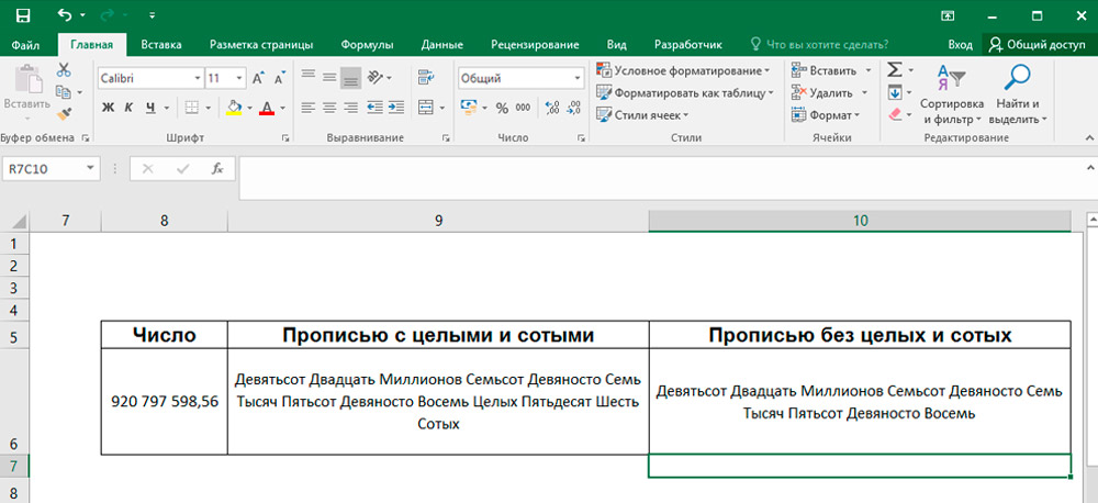
Now let’s see how to use this. Enter a number in the cell and click on the “Insert function” button. In the window that appears, select “User Defined” in the “Category” section. In the list below you will find the functions “Number in words”, “Sum in words” and several of its variations for currencies (rubles, hryvnia, dollars, euros). It is convenient to use if it is necessary to indicate any amount of money in words, which is very often required in various documentation.

Please note that after you have applied the function to a cell, all numbers that you enter into it will be immediately converted to text. Use “Number in words” or “Amount in words” depending on what tasks you face now.

As you can see, there is nothing difficult. Thanks to the ability to install extension packs, you can significantly increase the functionality of the program. By learning how to use the power of Microsoft Excel correctly, you will significantly increase your efficiency, saving you several hours of painstaking work. Write in the comments if the article was useful for you and ask questions that you might have in the process.