If the majority of computer users have a sin in half owning the Word text editor, then things are not so rosy with the equally famous spreadsheet processor. Many people simply do not see how this program can be used for everyday needs until they are faced with the need to perform calculations on large data samples.
But here, too, there are problems: not understanding the principles of Excel without outside help, users give up this lesson and never return to it.

Today’s article is intended for both categories of the population: simple step-by-step instructions will allow you to get started with the practical development of the program. Indeed, in fact, Excel allows you not only to perform calculations in a tabular view – the application can be used to draw up charts, multifactorial graphs, detailed reports.
Yes, tables in Word and Excel are completely different things, but in reality, working with tabular data is not at all difficult. And you don’t have to be a programmer for that.
Contents
Beginning of work
Practice is the best way to gain basic skills in any profession. Microsoft’s spreadsheet is no exception. This is a very useful application applicable in a wide variety of areas of activity, allowing you to organize fast calculations regardless of the amount of initial data.
Having mastered Excel, you are unlikely to become an expert in relational databases, but the skills acquired will be enough to achieve the status of “confident user”. And this is not only moral satisfaction and a way to show off to friends, but also a small plus to your resume.
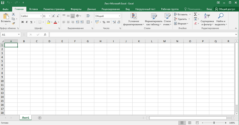
So, first, let’s take a look at the basic terms related to Excel:
- a table is a two-dimensional representation of sets of numbers or other values arranged in rows and columns. Line numbering is numeric, from 1 to infinity. For columns, it is customary to use letters of the Latin alphabet, and if you need more than 26 columns, then the Z will be followed by the indices AA, AB, and so on;
- thus, each cell located at the intersection of a column and a row will have a unique address such as A1 or C10. When we work with tabular data, the cells will be accessed by their addresses, or rather, by address ranges (for example, A1: A65, the separator here is a colon). In Excel, the table cursor does not bind to individual characters, but to the cell as a whole – this simplifies data manipulation. This means that with the cursor you can move around the table, but not inside the cell – there are other tools for this;
- a worksheet in Excel is understood as a specific table with a set of data and formulas for calculations;
- a workbook is a file with the xls extension, which can contain one or more worksheets, that is, it can be a set of related tables;
- you can work not only with individual cells or ranges, but also with their entirety. Separate elements of the list with semicolons (B2; B5: B12);
- using such indexing, you can select individual rows, columns or rectangular areas;
- various manipulations can be performed with table objects (copying, moving, formatting, deleting).
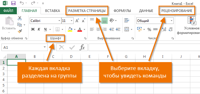
How to work with Excel: a beginner’s guide
So, we have received a certain minimum of theoretical information that allows us to proceed to the practical part. Now let’s take a look at how to work in Excel. Of course, after starting the program, we need to create a table. This can be done in different ways, the choice of which is carried out taking into account your preferences and your tasks.
Initially, we have an empty table, but already divided into cells, with numbered rows and columns. If we print out such a table, we get a blank sheet, without frames and borders.
Let’s figure out how to work with table elements – lines, columns and individual cells.
How to highlight a column / row
To select a column, click on its name, represented by a Latin letter or a combination of letters.
Accordingly, to select a line, you need to click with the mouse on the number corresponding to the required line.
To select a range of rows or columns, proceed as follows:
- right-click on the first index (letter or number), while the row / column will be highlighted;
- release the button and place the cursor on the second index;
- while holding down Shift, right-click on the second number / letter – the corresponding rectangular area will become selected.
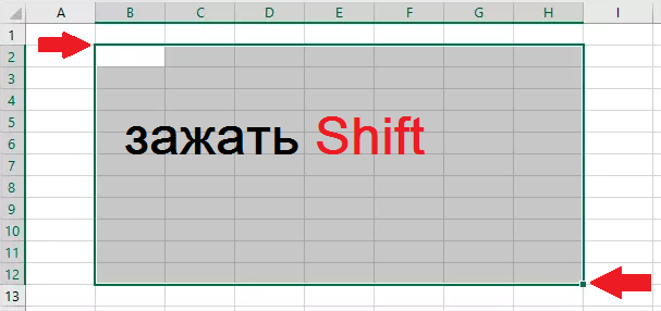
Highlighting lines using hot keys is performed by the Shift + Space key combination; to select a column, place the cursor in the desired cell and press Ctrl + Space.
Changing cell borders
Users who are trying to learn how to use Excel on their own often encounter a situation when content that exceeds its size is entered into a cell. This is especially inconvenient if it contains long text. There are two ways to extend the right border of a cell:
- manually, by clicking the left mouse button on the right border on the line with indices and keeping it pressed, move the border to the required distance;
- There is also an easier way: double-click on the border, and the program will independently expand the length of the cell (again, on the line with the letters-indices).

To increase the line height, you can click the “Wrap text” button on the toolbar, or drag the mouse over the border on the numeric index panel.
The Distribute Vertical button can be used to display text that does not fit in a cell on multiple lines.
Cancellation of the changes made is done in the standard way, using the “Cancel” button or the CTRL + Z combination. It is advisable to do such rollbacks right away – then it may not work.

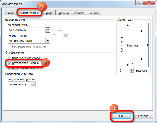
If you want to mark the formatting of the lines, you can use the “Format” tab, in which you select the “Auto-fit line height” item.
To cancel the changes in the column sizes, in the same tab “Format”, select the item “Width by default” – remember the number standing here, then select the cell, the borders of which have been changed and they need to be “returned”. Now go to the item “Column width” and enter the default value recorded in the previous step.
How to insert a column / row
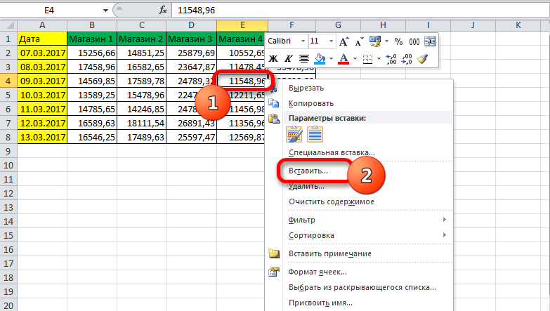
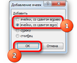
As usual, a row or column can be inserted in two ways, by calling the context menu with the mouse or by using hot keys. In the first case, right-click on the cell that needs to be moved, and in the menu that appears, select the item “Add cells”. A standard window will open in which you can specify what exactly you want to add, and it will be indicated where the expansion will take place (columns are added to the left of the current cell, rows are added at the top).
The same window can be called by the combination CTRL + SHIFT + “=”.
Such a detailed description of how to use the Excel program will undoubtedly come in handy for dummies, that is, beginners, because all these manipulations are in demand very often.
Step by step creation of a table, insertion of formulas
Usually, the first top row with index 1 contains the names of the fields or columns, and the rows contain separate entries. Therefore, the first step in creating a table is to put down the names of the columns (for example, “Product name”, “Invoice number”, “Buyer”, “Quantity”, “Price”, “Amount”).
After that, we also manually enter the data on the table. Perhaps, in the first or third column, we will have to push the boundaries – we already know how to do this /.
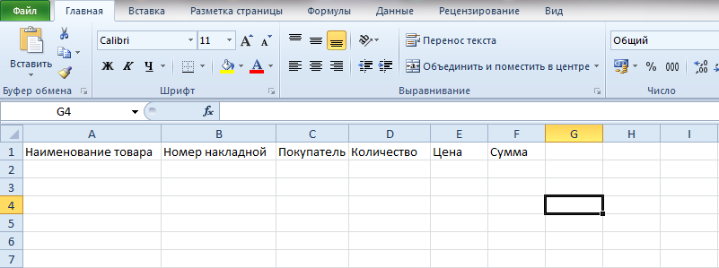
Now let’s talk about calculated values. In our case, this is the “Amount” column, which is equal to the multiplication of the quantity by the price. In our case, the “Amount” column has the letter F, the “Quantity” and “Price” columns – D and E, respectively.
So, we put the cursor in cell F2 and type the symbol “=”. This means that all the cells in column F will be calculated according to a formula.
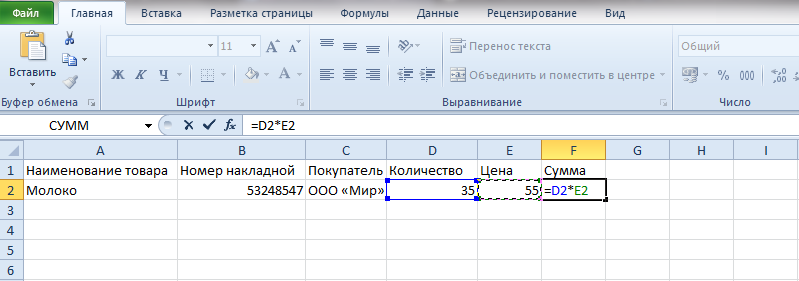
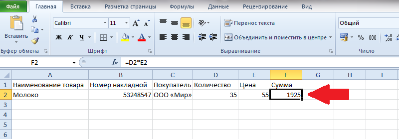
To enter the formula itself, select cell D2, press the multiply symbol, select cell E2, press Enter. As a result, cell D2 will contain a number equal to the product of the price and the quantity. To make the formula work for all rows of the table, click the lower left corner with the mouse in cell D2 (when you hover over it, a small cross will appear) and drag it down to the end. As a result, the formula will work for all cells, but with its own data set, taken in the same row.
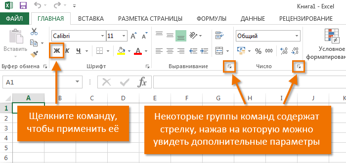
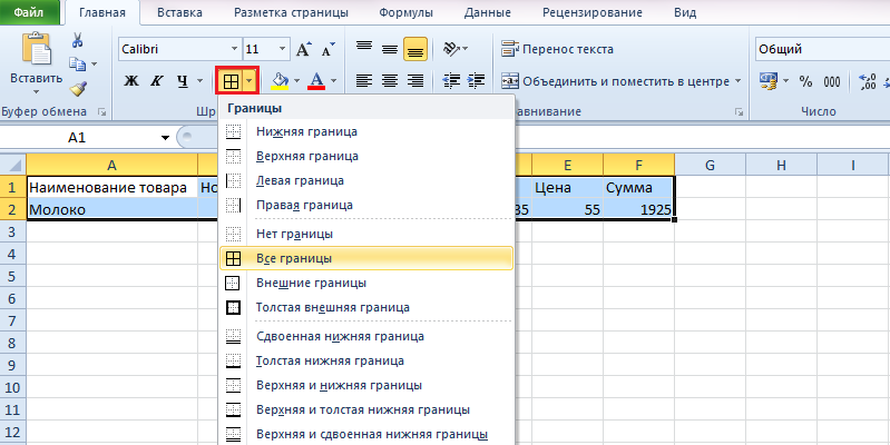
If we need to print a table, then to give a readable look, the rows and columns need to be constrained by a grid. To do this, select a section of the table with data, including the row with the names of the columns, select the “Borders” tab (it is located in the “Font” menu) and click on the symbol of the box with the words “All Borders”.
The Font tab allows you to format fonts in the same way as WTO and in Word. So, it is better to design the header in bold, text columns are better aligned to the left, and numbers are centered. So, you’ve got your first skills on how to work in Excel. Now let’s move on to considering other features of the table processor.
How to work with an Excel spreadsheet – a guide for dummies
We have considered the simplest example of tabular calculations, in which the multiplication function was entered manually in an inconvenient way.
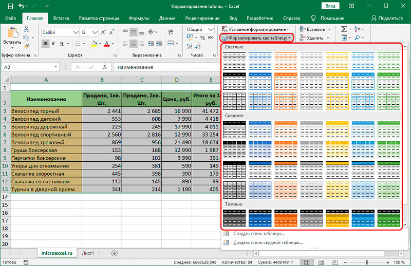
Creating tables can be made easier by using a tool called Design.
It allows you to assign a name to the table, set its size, you can use ready-made templates, change styles, it is possible to create rather complex reports.
Many beginners cannot figure out how to correct the value entered into a cell. When you click on a cell to be changed and try to enter characters, the old value disappears, and you have to enter everything all over again. In fact, the value of the cell when you click on it appears in the status bar located under the menu, and it is there that you need to edit its contents.
When entering the same values into cells, Excel shows intelligence, like search engines – it is enough to type a few characters from the previous line so that its contents appear in the current one – all you have to do is press Enter or go down one line below.
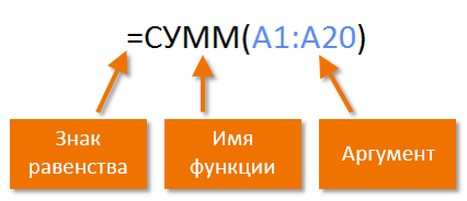
Excel function syntax
To calculate the totals for a column (in our case, the total amount of goods sold), you need to put the cursor in the cell in which the total is reported, and click the “AutoSum” button – as you can see, nothing complicated, quickly and efficiently. The same result can be achieved by pressing the combination ALT + “=”.
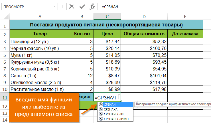
It is easier to enter formulas in the status bar. As soon as we press the “=” sign in a cell, it appears in it, and there is an arrow to the left of it. By clicking on it, we will receive a list of available functions, which are divided into categories (mathematical, logical, financial, working with text, etc.). Each of the functions has its own set of arguments that will need to be entered. Functions can be nested, when you select any function, a window with its brief description will appear, and after clicking OK, a window with the necessary arguments will appear.
After completing the work, when you exit the program, it will ask if you need to save the changes you made and will prompt you to enter a file name.
We hope that the information given here is enough to compile simple tables. As you master the Microsoft Excel package, you will learn its new features, but we affirm that you will hardly need a professional study of a spreadsheet processor. On the web and on bookshelves, you can find books and manuals from the For Dummies series on Excel for thousands of pages. Will you be able to master them in full? Doubtful. Moreover, you will not need most of the package’s features. In any case, we will be happy to answer your questions regarding the development of the most famous spreadsheet editor.