Sorting in Excel is a function built into the Microsoft Office suite that allows you to carry out analytical research and quickly find the required indicators. If you thoroughly learn how to do sorting in Excel, many data analysis tasks will be performed quickly and with absolute precision.
Contents
Sort by specified numeric values
Analysis of the work done, sales volumes, profit growth, student performance, purchases of additional materials are accompanied by the selection of parameters that have maximum and minimum indicators. Of course, if the table is small, then the user will be able to just find the best indicator. But in cases where Excel has an excessively large number of rows and columns, without using the built-in functions that allow you to sort the table, you can find the desired indicator, but you will have to spend a lot of time.
You can do much more practical, familiarize yourself with the information on how to sort in Excel, and immediately begin to practice the knowledge gained.
Ascending and descending filter
Sorting data in ascending or descending order is easy. It is only necessary to find out if the table is accompanied by numerous formulas. If this is the case, then it is best to transfer the table to a new sheet before sorting the data, which will avoid violations in the formulas or accidental breaking of links.

In addition, a fallback version of the table never hurts, because sometimes, getting confused in your own reasoning, wanting to return to the original version, it will be difficult to do this if you do not create a preliminary copy.
So, first you need to select the table to be analyzed. Next, go to a new sheet, right-click, and then click on the “Paste Special” line. A window with parameters will appear on the screen in front of the user, among which you need to select the “Value” parameter, and then click “OK”.

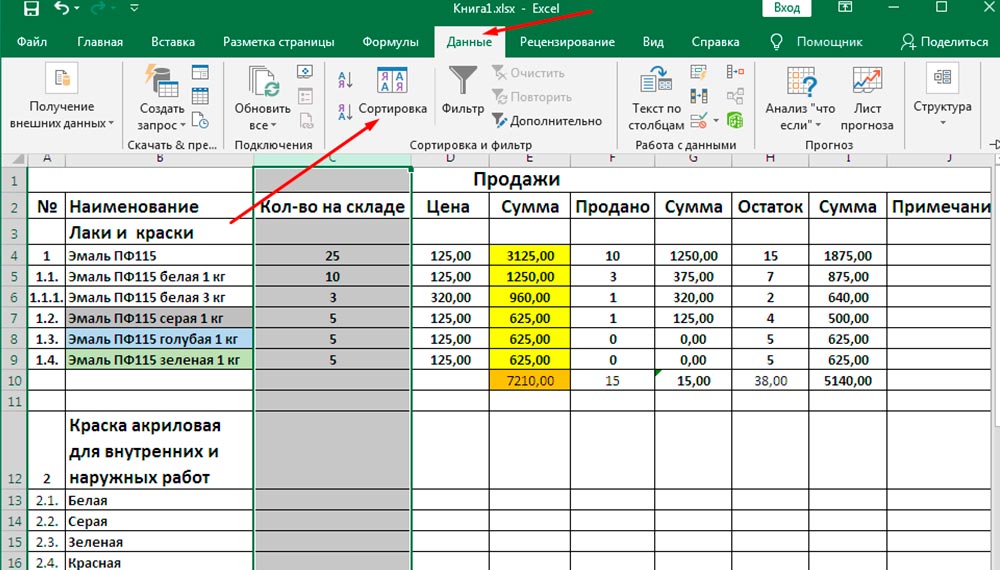
Now the duplicate variant has been created, so you can proceed with further actions. To fully understand how to sort a table in Excel in ascending order, you need to select the entire table again, then go to the “Data” tab, there, among several tools, there will be the desired “Sort” on which you need to click.

In the opened parameters window there is a line “My data contains headers”. There is a small window next to it, in which you should put a tick. It remains to put in the below opened windows the column to be analyzed, as well as the option of the desired sorting: ascending or descending. Next, we agree with the set parameters, after which the table will instantly demonstrate the desired result, saving you from hours of exhausting work.

If it is necessary to sort not in the whole table, but only in one column, the actions will be almost the same, except for only two points. Initially, you should select not the entire table, but only the desired column, and later, when Excel prompts you to automatically expand the range in order to sort, you need to refuse this by checking the box next to the phrase “Sort within the specified range”.
Sorting by other parameters
Sometimes, working in Excel, it becomes necessary to sort not numerical values in ascending or descending order, but somewhat different parameters, so you can read the practical advice of experienced users, thanks to which it is easy to figure out how to sort by date or by cell format in Excel.
Setting a filter by date and format
The sorting principle remains essentially the same. The user needs to select the table, specify the column to be analyzed, and then click on one of the suggested actions: “Sort from old to new” or “Sort from new to old”. After such actions, the table will sort all information or data by date.

Sometimes it is very important to do this again. This feature is built into the table. There is no need to re-enter several desired parameters, just click on the “Repeat” element in the filter.
Sometimes the filter can fail, but the reason is most likely incorrect display of some formats. In particular, if in some cells the data is entered in a non-date format, the sorting will not be carried out quite correctly.
If there is an urgent problem to sort the table by cell format, initially it is also desirable to transfer it to a new sheet, only now, after right-clicking on the “Paste Special” line, you must select the “Formats” parameter. Then, not only all data will be transferred to the new sheet, but also the applied formats, and the formulas will again be excluded.
It remains to re-enter the filter, in its parameters, select sorting by the color of the cells, then in the color window that opens, select the color that, after sorting, should be at the top or bottom. After clicking on “OK” the table will give an instant result.

If something went wrong, you need to know how to reverse sorting in Excel using one of two simple steps. You can simply press several times two simultaneously pressed keys (Ctrl + Z) until the table returns to its original form. If a lot of actions have been taken, it is easier to cancel sorting in the second way, closing the table without saving, then reopen it and start working again.
The sorting task can also be performed by:
- multiple columns;
- lines;
- random sorting method;
- in a dynamic way.
All of these options should now be considered separately.
Multiple Columns
This is an excellent and convenient enough way to set the secondary sorting order of a document and its data in Microsoft Excel.
To implement the task, you need to set several conditions for the subsequent sorting.
- First open the menu called Custom Sort. Here, assign the first criterion for the procedure. Namely the column.
- Now click on the “Add Level” button.
- After that, the screen will display windows for entering the data of the subsequent conditions for sorting. They need to be filled in.
Excel provides an excellent opportunity to add multiple criteria at once. This allows you to sort the data in a specific order that suits the user.
How to sort lines
If you pay attention to the default sorting, you will notice one pattern. The procedure is done column by column, not row by row.
But in some cases it is necessary to sort the data exactly by rows. The functionality of the Excel program provides such an opportunity.
Here, the user will need to do the following:
- open the Custom Sorting dialog box;
- click on the “Parameters” button in this window;
- wait for a new menu to open;
- select the item “Range Columns”;

- press the “OK” button;
- wait for the return to the main menu of the sorting window;
- now the “String” field will appear here for its subsequent filling with the necessary conditions.
Nothing complicated. Just a few clicks, and the task is completed.
Random way of sorting
It is important to note that the built-in sort options in the spreadsheet program do not have functionality to sort the data randomly in a column.
But there is a special feature called RAND that solves this problem from Microsoft’s tool.
Suppose a user needs to randomly arrange a certain set of numbers or letters in a column. To do this, you need to do the following:
- place the cursor on the left or right, on the adjacent cell;
- in this line, write a formula in the form of RAND ();

- press the Enter button on the keyboard;
- copy this formula to the entire column;
- get a set of random numbers;
- sort the column using ascending or descending principle.
This will arrange the values in random order. The formula is suitable for working with different input data.
Dynamic sorting method
Applying the standard sorting method to tables, when the data in them changes, the table will lose its relevance. Therefore, in many situations it is important to ensure that the sorting changes automatically when values change.
For this, the appropriate formula is applied. Consider this with a specific example.
- There is a set of primes. They must be sorted in ascending order, from smallest to largest.
- Near the column to the left or to the right, the cursor is placed on the adjacent cell.
- The formula is written, which is represented as = SMALL (A: A. ROW (A1)).
- The range to use should be the entire available column.
- The “String” function will be used as the coefficient. And with a link to the first registered cell.

- Now you can change one digit to another in the available original range. The sorting will change automatically.
If it is necessary to sort in descending order, then the LARGE is prescribed instead of the SMALL.
Nothing complicated in principle. Even a beginner can easily cope with such a task.
The use of sorts is much more convenient than the use of manual input and distribution of data by rows and columns. But here everyone chooses for himself the best tools and methods for composing data in Excel.
So, working with a filter in Excel is not difficult. It is enough to sort the data once, relying on the recommendations, and then everything will become so clear that it will be easy for you to master the rest of the filter parameters on your own.